„TLS noise” változatai közötti eltérés
| 3. sor: | 3. sor: | ||
[[file:Ballistic_diffusive.png|600px]] | [[file:Ballistic_diffusive.png|600px]] | ||
| − | Next, we model the temporal fluctuations of the conductance based on the scattering on | + | Next, we model the temporal fluctuations of the conductance based on the scattering on dynamical defects in a point contact geometry following the theoretical models summarized in [Fredicikk]. Following Ref. [Fredicikk] we will refer such dynamical defects as two levele systems (TLSs), but actually these diffects may also fluctuate between more than two different structural arrangements, the main ingradient is that the scattering on thses defects varies with time. First we emphasize, that a point-contact, i.e. a small, nanometer-scale junction between macroscopic electrodes always acts as a magnifier, i.e. all the scattering processes happening in the vicinity of the junction have highly enhanced influance on the conductance, and therefore it is even possible to observe the temporal conductance fluctuations due to a single two level system [Ralph, Caro, Kaijsers]. On the other hand the processes happening far away from the junction have highly suppressed contribution to the conductance. For the sake of simplicity we model an orifice like point contact, i.e. an orifice with diameter d in an infinite isolating plane between two conducting electrodes (see Figure). Without any scattering in the junction region, this orifice like \emph{ballistic} point contact has a conductance of [Fredicikk] |
$$G_\textrm{ballistic}=\frac{2e^2}{h}M,\ M=\left(\frac{k_\textrm{F}a}{2}\right)^2,$$ | $$G_\textrm{ballistic}=\frac{2e^2}{h}M,\ M=\left(\frac{k_\textrm{F}a}{2}\right)^2,$$ | ||
| − | where M is the number of open conductance channels in the contact, $a$ is the radius of the contact and $k_\textrm{F}$ is the Fermi wavenumber. | + | where M is the number of open conductance channels in the contact, $a$ is the radius of the contact and $k_\textrm{F}$ is the Fermi wavenumber, and $G_0=2e^2/h$ is the quantum conductance unit. If a TLS is placed to the center of the orifice, i.e. an atom or a group of atoms can fluctuate between two or more metastable positions, the electrons will scatter on the TLS modifying the above ballistic conductance formula. If we consider the scattering on a single atom-sized structural defect, the correction of the conductance to the above formula is on the order of the quantum conductance unit, or smaller. The difference between the conductanses of the different states of the TLS is therefore |
| + | $\Delta G_\textrm{ballistic}=(2e^2/h)C$, where $C$ defines the amplitude of thetemporal conductance fluctuation in the units of $G_0$ for a single TLS positioned inside a ballistic point contact. If the TLS is placed further away from the contact, the fluctuation of the conductance decreases with a geometrical factor $K_\textrm{ballistic}$, $\Delta G_\textrm{ballistic}=G_0\cdot C \cdot K_\textrm{ballistic}$. According to the detailed calculations in Ref. [Fredicikk] this geometrical factor scales with the square of the solid angle at witch the orifice is seen from the position of the TLS. Simply speaking, the scattering on the TLS only modifies the conductance, if the electron passing through the contact arrives to the TLS, and after that it is scattered back through the contact (see figure). Following these considerations we use the following approximatation for K_ball | ||
| + | K_ball=1 if r<d, and K_ball=(d/r)^4 if r>d. (Note that the solid angle, at wich the orifice is seen from position r on the contact axis is \Omega_r~(d/r)^2.) (pontosítani, mert ez 4pi-re normált). In a diffusive contact there are several further scattering centers with an averge distance of the mean free path, l, so if d>>l the electrons follow diffusive trajectories even inside the junction (see fig. ...). In this case the conductance of the junction can also be calculated yielding the so-called Maxwell conductance, G_diff=\sigma *d, where \sigma=ne^2\tau/m, where \tau=l/v_F is the momentum relaxation time, v_F being the absolute vaue of the Fermi velocity. Expressing the electron density by k_F, one gets: G_diff=G_ball* (16/3\pi)*(l/d). If a single TLS is placed in a diffusive point contcact, the temporal fluctuation of the conductance is \Delta G_diff=2e^2/h * C*K_diff, where C still tells us the conductance fluctuation, if the TLS would be inside a ballistic junction, whereas K_diff is a geometrical factor characteristic for diffusive junctions. | ||
| + | |||
</wlatex> | </wlatex> | ||
A lap 2018. november 12., 11:01-kori változata

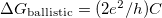
Next, we model the temporal fluctuations of the conductance based on the scattering on dynamical defects in a point contact geometry following the theoretical models summarized in [Fredicikk]. Following Ref. [Fredicikk] we will refer such dynamical defects as two levele systems (TLSs), but actually these diffects may also fluctuate between more than two different structural arrangements, the main ingradient is that the scattering on thses defects varies with time. First we emphasize, that a point-contact, i.e. a small, nanometer-scale junction between macroscopic electrodes always acts as a magnifier, i.e. all the scattering processes happening in the vicinity of the junction have highly enhanced influance on the conductance, and therefore it is even possible to observe the temporal conductance fluctuations due to a single two level system [Ralph, Caro, Kaijsers]. On the other hand the processes happening far away from the junction have highly suppressed contribution to the conductance. For the sake of simplicity we model an orifice like point contact, i.e. an orifice with diameter d in an infinite isolating plane between two conducting electrodes (see Figure). Without any scattering in the junction region, this orifice like \emph{ballistic} point contact has a conductance of [Fredicikk]
![\[G_\textrm{ballistic}=\frac{2e^2}{h}M,\ M=\left(\frac{k_\textrm{F}a}{2}\right)^2,\]](/images/math/c/9/a/c9a2f7766c9f70a9691b01f14c11e40f.png)
where M is the number of open conductance channels in the contact,  is the radius of the contact and
  is the Fermi wavenumber, and
  is the quantum conductance unit. If a TLS is placed to the center of the orifice, i.e. an atom or a group of atoms can fluctuate between two or more metastable positions, the electrons will scatter on the TLS modifying the above ballistic conductance formula. If we consider the scattering on a single atom-sized structural defect, the correction of the conductance to the above formula is on the order of the quantum conductance unit, or smaller. The difference between the conductanses of the different states of the TLS is therefore
 , where
  defines the amplitude of thetemporal conductance fluctuation in the units of
  for a single TLS positioned inside a ballistic point contact. If the TLS is placed further away from the contact, the fluctuation of the conductance decreases with a geometrical factor
  ,
,  . According to the detailed calculations in Ref. [Fredicikk] this geometrical factor scales with the square of the solid angle at witch the orifice is seen from the position of the TLS. Simply speaking, the scattering on the TLS only modifies the conductance, if the electron passing through the contact arrives to the TLS, and after that it is scattered back through the contact (see figure). Following these considerations we use the following approximatation for K_ball
K_ball=1 if r<d, and K_ball=(d/r)^4 if r>d. (Note that the solid angle, at wich the orifice is seen from position r on the contact axis is \Omega_r~(d/r)^2.) (pontosítani, mert ez 4pi-re normált). In a diffusive contact there are several further scattering centers with an averge distance of the mean free path, l, so if d>>l the electrons follow diffusive trajectories even inside the junction (see fig. ...). In this case the conductance of the junction can also be calculated yielding the so-called Maxwell conductance, G_diff=\sigma *d, where \sigma=ne^2\tau/m, where \tau=l/v_F is the momentum relaxation time, v_F being the absolute vaue of the Fermi velocity. Expressing the electron density by k_F, one gets: G_diff=G_ball* (16/3\pi)*(l/d). If a single TLS is placed in a diffusive point contcact, the temporal fluctuation of the conductance is \Delta G_diff=2e^2/h * C*K_diff, where C still tells us the conductance fluctuation, if the TLS would be inside a ballistic junction, whereas K_diff is a geometrical factor characteristic for diffusive junctions.
. According to the detailed calculations in Ref. [Fredicikk] this geometrical factor scales with the square of the solid angle at witch the orifice is seen from the position of the TLS. Simply speaking, the scattering on the TLS only modifies the conductance, if the electron passing through the contact arrives to the TLS, and after that it is scattered back through the contact (see figure). Following these considerations we use the following approximatation for K_ball
K_ball=1 if r<d, and K_ball=(d/r)^4 if r>d. (Note that the solid angle, at wich the orifice is seen from position r on the contact axis is \Omega_r~(d/r)^2.) (pontosítani, mert ez 4pi-re normált). In a diffusive contact there are several further scattering centers with an averge distance of the mean free path, l, so if d>>l the electrons follow diffusive trajectories even inside the junction (see fig. ...). In this case the conductance of the junction can also be calculated yielding the so-called Maxwell conductance, G_diff=\sigma *d, where \sigma=ne^2\tau/m, where \tau=l/v_F is the momentum relaxation time, v_F being the absolute vaue of the Fermi velocity. Expressing the electron density by k_F, one gets: G_diff=G_ball* (16/3\pi)*(l/d). If a single TLS is placed in a diffusive point contcact, the temporal fluctuation of the conductance is \Delta G_diff=2e^2/h * C*K_diff, where C still tells us the conductance fluctuation, if the TLS would be inside a ballistic junction, whereas K_diff is a geometrical factor characteristic for diffusive junctions.