Függvényillesztés Monte Carlo módszerrel mérésleírás
This page is outdated. Read the description of the lab exercise in Moodle.
Az alábbi leírás pdf formátumban is letölthető. Példa adatsor: Data.txt.
Tartalomjegyzék[elrejtés] |
Bevezetés
A Monte Carlo algoritmusok szerteágazó alkalmazási területei közül a függvényillesztés a számítógépes gyakorlat témája. A leírás áttekinti a szükséges elméleti hátteret, valamint segítséget ad a konkrét megvalósításhoz.
Elméleti háttér
Legyen az illesztendő adatsor , ahol
  . Az illesztett adatsor hasonlóan
  , ahol
  a paraméterek listája, amelyek hangolásával érjük el, hogy az illesztett adatsor rásimuljon az eredetire. Ez a következő energiakifejezés minimalizálását jelenti:
 ![\[E(\vec{A})=\sum_{i=1}^{N} \left| Y_\textrm{orig}(X_\textrm{i}) - Y_\textrm{fit}(X_\textrm{i}, \vec{A})\right| \label{MCEnergyEq} \]](/images/math/b/c/9/bc95522349a8e6ac1157fbcc34e08ad7.png)
A minimalizálást Monte Carlo--Metropolis algoritmussal végezzük: Változtassuk meg a paramétereket véletlenszerűen:  . Ezzel a fentiek szerint kiszámolt energia is változik:
  . Az új paramétereket elfogadjuk, ha közelebb kerültünk a minimumhoz, tehát
  . Célunk elkerülni, hogy az algoritmus befagyjon egy lokális minimumba, ezért
 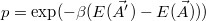 valószínűséggel dolgozunk tovább az új paraméterekkel, ha
  . Vegyük észre, hogy
  esetben csak lefelé léphetünk, míg a
  határátmenetben véletlenszerű mozgást kapunk a paramétertérben. Ez adja a fizikai jelentését az algoritmusban szereplő
  értéknek: megfeleltethető egy, a paramétertérben mozgó részecske
  inverz hőmérsékletének.
Implementáció
A fentiek megvalósításához a következő felépítést érdemes követni:
- Készítsünk globális tömböt az eredeti, valamint az illesztett adatsornak;
- Hasonlóan globális változókban tároljuk az inverz hőmérsékletet, az illesztési paramétereket, valamint azok lépésközét;
- Deklaráljunk egy véletlenszám-generátort: a paraméterek megváltoztatásához és az
 valószínűségű lépéshez (csak egyszer hozzuk létre a Random() objektumot, és csak egy példányt);
- Hozzunk létre globális változókat a megváltoztatott paramétereknek, valamint egy tömböt a megváltoztatott paraméterekkel generált illesztőfüggvénynek.
Az illesztés inicializálásához hozzuk létre a szükséges változókat, és olvassuk be a kezdőértékeket a TextBoxokból.
Az illesztést az alábbiak szerint végezzük:
- Számítsuk ki a
 szerinti energiát az aktuális változókkal;
- Változtassuk meg az egyik paramétert a megadott határok között egyenletes eloszlással;
- Számítsuk ki az így megváltozott energiát;
- A régi és új energia különbsége alapján döntsünk arról, hogy elfogadjuk-e a változást: ha az új érték kisebb, akkor minden esetben, ha nem, akkor sorsoljunk egy véletlenszámot, és valószínűséggel mégis elfogadjuk a változást;
- Ha szükséges, írjuk ki az új értéket a TextBoxba, és ábrázoljuk a megváltozott illesztőfüggvényt;
- A fentiek szerint járjunk el a többi paraméter esetében.
Feladatok
Készítsünk grafikus függvényillesztő felületet a data.dat file-ban található 500 elemű adatsor illesztéséhez a![\[ y(t)=Ae^{-t/\tau}\sin(2\pi t/T)\]](/images/math/4/f/0/4f0332aa1420c838cd15b43a82ebe856.png)
 a keresett paraméterek. A cél eléréséhez az alábbiak szerint haladjunk:
- Olvassuk be és ábrázoljuk a data.dat állomány tartalmát!
- Hozzunk létre TextBoxokat, amelyekkel állíthatóak a függvényillesztés kiinduló paraméterei, azok lépésköze, valamint az inverz hőmérséklet!
- Hozzunk létre gombokat, amelyekkel elindíthatjuk a függvényillesztést: legyen lehetséges újraindítani az illesztést a TextBoxokban megadott kezdeti paraméterekkel, valamint 1, illetve N (TextBoxban megadható) illesztési ciklust elindítani!
- A program jelenítse meg az aktuális paramétereket, az szerinti energiát, valamint az illesztett függvényt!
- Célszerű egy külön grafikonon ábrázolni az előző értékeit lépésszám függvényében. Ezen szemmel könnyen áttekinthető az algoritmus konvergenciája.
A jegyzőkönyvben szerepeljen a program felépítésének leírása, valamint a probléma diszkussziója. Vizualizáljuk az skalárteret alacsonyabb dimenziós (1D és 2D) metszeteken keresztül. Vizsgáljuk meg a kezdeti paraméterek, az inverz hőmérséklet, valamint a paraméterek lépésközeinek hatását az illesztés gyorsaságára és jóságára. Grafikonon ábrázoljuk, az inverz hőmérséklet néhány nagyságrendnyi függvényében, hogy átlagosan hány lépés után illeszkedik a generált függvény az eredetire, valamint mekkora a jellemző minimális energia (átlagoljuk ki több illesztési próbálkozásból).
Opcionálisan próbáljuk ki, hogy lehetséges-e jobb eredményt elérni, ha -t, illetve a lépésközöket dinamikusan változtatjuk! A dokumentációhoz csatoljuk a program forráskódját!
Syllabus in English
The exercise sample data is available here: Data.txt.
Introcution
Monte Carlo algorithms have a widespread use in many fields, this exercise focuses on fitting a function to a series of data (such as what would be obtained by an experimental measurement). The exercise description presents the necessary theoretical background, and provides indications for the concrete implementation.
Theoretical background
, where . The fitted data series is , where is the list of parameters that are varied to obtain the best correlation between the fitted series and the original series. The best fit is to be regarded as a minimization of the following "energy" expression: The minimization of energy is obtained through the Monte Carlo - Metropolis algorithm: First, alter the fitting parameters with a random factor: . Using the new randomly varied parameters, a new energy value is obtained: . The new parameters should be accepted and kept, if the new energy is closer to the energy minimum, that is, . The key to the algorithm is to avoid becoming stuck in a local minimum, thus we use an "annealing" method, where with probability we accept the new parameters, even if . Observe that using the algorithm can only step downwards in energy, while in the limit the walk in the parameter space is entirely random. This gives a physical meaning to the value: it can be regarded as particle moving in the parameter space with inverse temperature.
Implementation
To create the program with the above considerations, follow these steps:
- Create a global variable array for both the original and fitted data series.
- Also in global variables, store the inverse temperature, the fitting parameters, and their maximum random increment;
- Create a random number generator for the parameter variation and for the probability acceptance step (make only a single Random() instance, and make it only once);
- Create global variables to temporarily store the randomly altered parameter set and a data series generated by this set. This is needed so that reverting to the previous parameter set and series is possible in case a new parameter set is not accepted.
To initiate the fitting, initialize the required variables, and read the starting values from TextBoxes.
The steps in the fitting algorithm are the following:
- Calculate energy using the current fitted series;
- Alter one of the parameters within the specified limits with a uniform random distribution;
- Calculate the new energy;
- Based on the difference between the new and previous energy, decide to accept the parameter change: If the new value is smaller, then accept it; if not, then get a new random value between 0-1, and with probability accept it anyway; otherwise discard it;
- If necessary, display the new values in a TextBox and display the altered fitting function on graph;
- Repeat these steps for every other parameter as well.
Tasks
Create a graphical interface for controlling the fitting program. Use the provided data.txt as an input, having 500 elements in the data series. The fitting is to be attempted using the are the parameters to find. To obtain the best fit, proceed the following way:
- Read the data.txt file contents into your program's memory and display its contents!
- Create TextBoxes, for the user to set the starting parameters of the function, their random variation interval, and the inverse temperature!
- Create buttons to start the fitting algorithm: let it be possible to restart the fitting using newly introduced TextBox values, to execute 1 step of the algorithm, or to execute a user-defined number of steps (given in a separate TextBox).
- The program should display the current actual parameters, the energy , and on graph the fitted series in a separate color than the original data series!
- It is advisable to display, in a separate graph, the history of energy as a function of fitting steps done by the algorithm. This makes it possible to tell when the algorithm has converged to a minimum.
In the report, describe the workings of your program, and discuss the problem. Visualize the scalar field through lower-dimensional (1D and 2D) cross-sections. Describe, with examples given, how your program reacts when different starting parameters are given, when various inverse temperatures are used, or how the random variation interval of parameters affects the output of fitting. You should describe the performance of your program by considering the number of steps necessary to find the minimum with certain starting conditions, as well as compare the minimum energies obtained, to be able to tell if some conditions prevented your algorithm from finding the global minimum energy.
Optionally, try to check if you can get a better result (faster fit) if and and variation intervals are dynamically tuned! Attach the source code to your documentation!