Scanning tunneling microscope
Scanning Tunneling Microscope - STM
Even the ancient greeks suspected that matter consists of atoms. In the beginning of the 20th century this assumption could be proved by several measurements, yet to make a picture of the atoms on the surface of a material, we had to wait until 1981, when Gerd Binning and Heinrich Rohrer built the first scanning tunneling microscope (STM). In 1986 they won the Nobel Prize for their invention. Since then the scanning tunneling microscope is widely used, and nowadays it is one of the basic experimental devices in nanophysical research. Its working principle is based on tunneling effect: a sharp tip is positioned to a few nanometers from the surface of the investigated sample, then voltage is applied to the tip, which induces tunneling current between the tip and the sample:
![\[I \propto V_b \cdot \mathrm{Exp}\left\{-A\cdot d\cdot \sqrt{\Phi} \right\},\]](/images/math/f/3/3/f33f7d155ad3c25c2642a7c71de1f639.png)
where  is the potential difference between the sample and the tip, d is the sample-tip distance,
  is the work function, and
 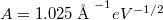 is a constant. As the tunneling current depends exponentially on the distance, a very precise measurement is possible: if we change the sample-tip distance with 1Å (which is approximately half the size of an atom), the current falls to its 1/10.
 |
| fig. 1: Approaching with tip to the surface, source: András Magyarkuti, master thesis defence, BUTE Department of Physics, 2013. |
In the beginning of the measurement the sample is approached with the tip (like it can be seen on fig. 1), until the current reaches a certain value (usually it has the order of magnitude of a few nA). The scanning tunneling microscope can be used in 2 ways: constant current or constant distance. The most frequently used is the constant current mode (fig. 2): in this mode the sample is scanned parallel to its surface with the tip, while measuring the tunneling current with a controlling circuit, and vertically moving the tip perpendicular to the sample, so that the measured tunneling current is constant, i.e. that the sample-tip distance remains approximately the same. This way the topography of the sample can be scanned with atomic resolution.
 |
| fig. 2: Scanning over the sample: recording the topography in constant current mode, source: András Magyarkuti, master thesis defence, BUTE Department of Physics, 2013. |
The other mode is the constant height mode (fig. 3): in this mode the control is turned off, and the sample is scanned with the tip in a fixed height. The topography of the sample can be determined from the measured tunneling current. This mode enables quick scanning, which can be particularly useful if some slow temporal change (like shifting caused by thermal expansion) needs to be eliminated. To use this mode, the sample has to be sufficiently smooth and the tip has to be far enough from the surface so it doesn’t crash into the sample.
 |
| fig. 3: Scanning over the sample: recording the topography in constant height mode, source: András Magyarkuti, master thesis defence, BUTE Department of Physics, 2013. |
The exponential dependence of the tunneling current on the sample-tip distance enables us to make high quality STM pictures using a tip sharpened by a pair of scissors. The figures below show atomic resolution pictures of the surface of a graphite sample and of a carbon nanotube.
 |
| fig. 4: STM picture of graphite surface with atomic resolution, source: András Magyarkuti, master thesis, BUTE Department of Physics, 2013. |
 |
| fig. 5: STM picture of a carbon nanotube, source: Wikipedia |
The STM tip cannot only be used for imaging but also for manipulating the sample with atomic resolution: atoms can be moved along the surface using the tip. The circular formation consisting of 48 iron atoms on a copper surface (seen on fig. 6) was made using this technique. On the picture made with a tunneling microscope the standing waves formed inside the circle can be well seen (“quantum corral”). In another similar experiment an ellipse consisting of 36 cobalt atoms was formed and a cobalt atom was added to one of the focal points; thanks to the wave nature of electrons, the effect of the cobalt atom can be observed in the other focal point as well. 1
 |
| fig. 6: Electron standing waves inside of circle built up from atoms, forrás: Wikipedia |
.jpg)
The STM setup
For the demonstrational STM the Smart Piezo Drive MK3-HV1 amplifier was used. This is a professional, three channel amplifier made for piezoelectric actuators, which has outputs that can vary in the -200 V to 200 V range. Applying  10 V to its inputs the output voltage can be controlled. As its outputs connected to the SoftdB MK2-A810 XYZ piezoelectric actuator can take a value from -10 V to 10 V. The block diagram of the STM setup can be seen on fig. 7.
 |
| fig. 7: The block diagram of the STM system, source: Botond Sánta, Pásztázó szondás mérőrendszer fejlesztése, master thesis, BUTE Department of Physics, 2016. |
How to use the GXSM
To operate the STM a complex operating and controlling system is necessary. This system’s most important tasks are: the control of the position of the tip according to the tunneling current measurements; recording and displaying the tunneling current; changing the piezo voltage in the scanning process; and every other function that enables the operation of the STM.
The MK2-A810 SPM controller used in this STM setup has 8 analog inputs/outputs capable of operating at a sampling rate up to 150 kHz with a 10V dynamic range. Besides that 16 individually configurable digital inputs/outputs and 2 16-bit counters inputs are also available. The circuit has a very low noise level and a high DC stability for every channel, which are crucial for the operation of the STM. A big advantage of this hardware is its compatibility with the open source GXSM SPM controller software. The GXSM software (Gnome X Scanning Microscopy) is a controlling and data processing software, which was written for Linux environment, and can be used for any kind of scanning probe microscope. As this is an open source software, its elements can be changed according to the users preferences, which enables the extensive usage of the software and the realization of special measurements. The most important functions of the GXSM software can be seen on fig. 8, highlighting the functions of each window.
 |
| fig. 8: The most important functions of the GXSM software, source: Botond Sánta, Pásztázó szondás mérőrendszer fejlesztése, master thesis, BUTE Department of Physics, 2016. |
The GXSM is able to display any channel, which was configured as an input. During a scanning process usually the topography and the tunneling current are displayed both for the forward and backward movements of the tip. If the 2 topographies recorded by the forward and backward moving tip are approximately the same, the imaging (which is influenced by the tip quality) is good. The GXSM software enables the usage of the PI controlling method, which is a widely used method in industrial control systems. The essence of this method is, that we enter an arbitrarily chosen tunneling current target value:  (setpoint), then we write the
 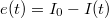 error. Using this notation the derivative of the voltage applied to the
  -piezo can be written as:
![\[ \dot{z}(t)=C_p \cdot e(t) + C_i \int_0^t e(\tau) d\tau, \]](/images/math/e/6/1/e6134a2570a126078da709be525613de.png)
Where  is the proportional and
  the integral coefficient, which are dimensionless. These two values determine the time constant (
 ) of the PI control:
![\[ \tau_{PI} = \frac{C_p}{C_i} \]](/images/math/5/5/2/552c83775db2e9436a6b8e32b3fc3617.png)
The lower the time constant, the quicker the control. The GXSM software uses its control parameters in unusual units, so the time constant of the control can be calculated as:
![\[ \tau_{PI} = \frac{C_p}{75000} \cdot C_i \]](/images/math/a/f/e/afef33515b6cbac63b26e6337f7677f0.png)
The typical values in the measurements are:  and
and  , though these can be different according to the details of the experiment, especially for unstable measurements.
 |
| fig. 9: Scanning funtions of the GXSM software, source: Botond Sánta, Pásztázó szondás mérőrendszer fejlesztése, master thesis, BUTE Department of Physics, 2016. |
Measurement tasks
- Place a vacuum evaporated gold sample into the sample holder. Make sure that every connection is secured (it didn't break off, every connection is attached.)
- Start the coarse approaching of the sample with the tip manually, using an optical microscope. Approach the sample until the tip and its reflection get so close to each other that they almost touch. (But they must not touch each other.)
- Run the GXSM program on the computer with the Linux operating system.
- In the window SR DSP Control\Advanced check the Enable Feed Back Controller, and the Internal Offset Adding options.
- In the SR DSP Control \ Feedback & Scan window set the piezo gain values to 20 (at the bottom of the window).
- Set the control of the stepping motor in the GXSM:
- Mover control\ Config: X-motor, Pulse: positive
- Mover control\ Auto: Amplitude = 5 V, Duration = 1 ms,
- Try the manual control using the > button that can be found at the bottom of the Mover control\Auto window. Now we must see on the recording made with a microscope, that the tip starts moving. The direction in which the motor is rotating is determined by the DIR switch positioned on the side of the box of the controlling circuit. It is NOT determined by the program! If we want to move the tip backwards, we must not use the < button but change the direction using the DIR switch & move using the > button.
- Use the automatic approach to move the tip to an atomic distance from the sample.
- In the SR DSP Control \ Feedback & Scan window set the following settings: Bias = 1V, Scurrent = 0,7-2 nA, ScanSpd = 1000-2000
 !
!
- Set the Max steps to a value between 1 and 5 at the Mover Control\Auto menu, and push the button below the label Auto Control.
- In the SR DSP Control \ Feedback & Scan window set the following settings: Bias = 1V, Scurrent = 0,7-2 nA, ScanSpd = 1000-2000
The automatic approach can be stopped using the red X button below the label Auto Control. In case the AutoApproach function is not working or Scurrent is set to 0 (i.e. no tunneling current was given, and the approach does not start), or the signal is too noisy, then the Scurrent value should be changed to a higher one (but maximum to 2.5 nA!).
Calibration
- Make a calibration to know the relation between the voltage applied to the piezo actuator and the real physical displacement.
- Using the GXSM program distance the tip from the surface of the sample while recording the tunneling current as a function of time.
In the SR DSP Control set the followings: Z-Start = 0  , Z-End = 30 , Points = 250, Z-slope = 10 , Slope-ramp = 10 , Auto Plot.
- By clicking the Execute button, the program starts distancing the tip according to the parameters set previously, and plots the tunneling current as a function of time. It is worth to change to logarithmic scale on the plot. Record current and the Z-piezo voltage as a function of time using the other computer with the Windows operating system.
- We can plot the measured current (the gain of the Femto is 1 nA/V) and fit a line to the logarithm of the current.
- Using to the equation given in the theoretical introduction calculate the distance of the electrodes corresponding to the tunneling current. Applying this calibration, the Z-piezo voltage can be converted to displacement in the following measurements.
Stability measurements
- Measure long-term STM stability!
- Measure the stability using the Minus-K vibration isolation table.
- Let’s measure the effect of the PI parameters on the stability of the system. Save some curves using different P & I parameters, including at least three cases: optimal parameters, too slow and too fast feedback. Plot the the tunnel current and the displacement over time, along with the relative standard deviation for each cases.
- Display current on a logarithmic axis, and calculate the displacement from the acquired stability according to the previous calibration (i.e. the accuracy of the tip-sample distance sustained by the controlling circuit)! (Displacement can be calculated from the piezo gain and the sensitivity of piezo actuators also.)
Thermal excitations
- Investigate the thermal stability of the system!
- Wait until the system reaches thermal equilibrium!
- Heat the system using infrared light and record the voltage applied to the piezo actuator as a function of time. Perform the experiment so, that the measured data also includes a part of the cooling of the curve.
- Calculate the physical displacement caused by the thermal expansion, according to the calibration.The sensitivity of all piezo actuators used in the setup is
 . Compare your result with the theoretical estimation (i.e. how large the thermal expansion in the given system can be.)
Mechanical excitations
- Excite the stable STM system with applause!
- Record a few stability curves while applauding a few times.
- Explain what you see.
- Excite the system with pounding on the ground.
- Pound on the ground next to the STM system and record the stability traces.
- Compare the two excitations and discuss the results!
- Toss the vibration isolation table!
- Carefully(!) toss the vibration isolation table in horizontal and vertical directions.
- Record the damped oscillation.
Scanning
- Scan the vacuum evaporated gold sample.
- In the Channel Selector window set the followings: Mode\Topo and DIR\->, and in the 2nd row: Mode\Topo and DIR\<-.
This way we see the topography during the scan in two windows: one of them shows the recorded topography while scanning in one direction, and the other one shows the topography recorded while scanning inn the opposite direction. The two figures must be each others reflections in case of an ideal tip. Any difference can be explained as a consequence of the imperfections of the tip.
- In the GXSM - STM/AFM/SPA-LEED... window the following settings can be changed:
- Range XY - X & Y dimensions of the scanned window, given in units of nm.
- Points XY - Determines the resolution of the window, i.e. the dimensions of one datapoint (e.g.: for a window with dimensions of 100x100 nm and the resolution is set to a value of 100x100 points, then the size of one datapoint is an average value over a surface with dimensions of 1 nm).
- Offset XY - As the default setting the program places the tip in the middle of the maximal scannable window (for the given configuration the size of the scannable window is 2400 x 2400 nm). This means, that the tip can move half of the maximal piezo displacement (1200 nm) in both directions. In case we are not interested in the middle, but in another part of the window, it is useful that the default position of the tip can be changed using this option. It is important to note, that this function is always used in serious measurements, because when using the Autoapproach function, it often happens that the tip is crashed into the middle of the scannable window, damaging the sample in the middle.
- Rotation - As the default setting the tip moves from left to right, then right to left (this is the so called linescan), after the line is scanned the tio jumps down a bit, and continues the scan. This is the 0° setting. In some cases (e.g. for samples with special structures, like grooves) it might be useful to change the direction of the scan. A value between 0-360° can be entered.
- Scan button - Start a single scan. After the scan is finished, the tip returns automatically to the default position (which might have been changed by the Offset XY function).
- Movie button - Start the continuous scanning. After a scan is finished, the process is repeated from the beginning. The process can only be stopped using the Stop button!
- Stop button - Stop the scanning any time. The tip returns automatically to the default position (which might have been changed by the Offset XY function).
- Save button - Save the displayed channels (TOPO, ADC0, stb.).
- Exit button - Exit the GXSM program.
- In the GXSM - STM/AFM/SPA-LEED... window the following settings can be changed: