Lock-in programming, investigation of a quartz sensor
Purpose of the measurement
The purpose of this measurement is to learn the usage and programming of the Stanford Research Systems SRS830 digital lock-in amplifier. For this purpose you're going to do a test measurement on an LC circuit, then you'll investigate and characterize a quartz sensor similar that can be used in atomic force microscopy (AFM) devices.
Nanophysical application of quartz oscillators used in watches
A quartz resonator used in quartz clocks is shown in the left side of Figure 1. Similar devices are being used to generate clock signal in electronic circuits, their most important parameter is their resonance frequency. The tuning fork (TF) shaped oscillator in the Figure has a nominal resonance frequency of 32 768 Hz (= 215 Hz).
Due to the piezoelectric properties of crystalline quartz the oscillation of the tuning fork can be excited by electric voltage. Of course, a body shaped like this has several vibration modes, but the electrodes are made such way they mainly excite the mode where the prongs of the tuning fork stay in their plane and their leaning is symmetric in a way their displacements are opposite. During a vibration in this mode there are no force or angular momentum acting on the foot piece of the TF, so it is only weakly coupled to its environment. Therefore it can keep its resonance even in wristwatches where it is exposed to rapidly changing acceleration.
While applying AC voltage to its electrodes the deformation of the crystal is being periodic, it starts to vibrate. When the frequency of the applied voltage equals to the resonance frequency of the crystal, the amplitude of the vibration can be extremely high. For the detection of the vibration one measures the current between the electrodes which is proportional the velocity of the prongs of the tuning fork. This current has a maximum value at the resonance frequency illustrated by the resonance curve in the right side of Figure 1.
 |
 |
| Figure 1. A quartz resonator used in watches (left) and its resonance curve (right). This curve is the amplitude of the current of the device in the function of the frequency of the constant amplitude excitation voltage. Source: András Magyarkuti MSc thesis (BME, Department of Physics, 2013, in Hungarian). | |
In a conventional atomic force microscope a sharp tip is placed at the and of a cantilever, then it is approached to the surface of a sample. The movement of the cantilever is usually detected by a laser beam reflected from its other side. In dynamic mode a vibration in the cantilever is excited near to its resonance frequency. When the tip is close to the sample, due to the force between the surface and the end of the tip, the resonance frequency of the cantilever is different than it would be during free vibration. While sweeping the tip over the sample in x and y directions the z height of the cantilever is being continuously adjusted in a way the resonance frequency of the vibration is constant, so are the force and distance between the sample and the tip as it is shown in the video of Figure 2. (Note that the change in resonance frequency is not proportional to the force but to the spring constant of the system which is proportional to the derivative of the force respect to the distance of the tip and the sample.) Since the z height of the tip is known (it is controlled by us) its dependence on the x and y positions gives the topography of the sample even in atomic resolution.
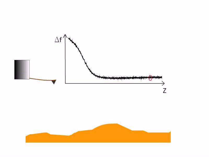 |
| Figure 2. The principle of atomic force microscopy in non-contact dynamic mode. Source: András Magyarkuti MSc defence (BME, Department of Physics, 2013). |
During low temperature AFM measurements the optical detection of the cantilevers movement is very challenging. Therefore it is practical to use a sensor which movement can be measured in an electrical way. The simple and cheap quartz tuning fork shown in Figure 1. is suitable to be used in an AFM device by attaching a sharp tip on one of its prongs because of the high quality factor of its resonance which ensures that a small force on the tip causes a measurable change in the resonance frequency. It is demonstrated in Figure 3. On the left side there is scanning tunneling microscope (STM) image of a gold coated nanostructure (the height of the tip was adjusted in a way that the tunneling current was constant), on the right side the same area was mapped with a tuning fork keeping the force (and the resonance frequency) constant between the sample and the tip. The main features of the two images are matching.
 |

|
| Figure 3. The topography of a gold coated surface measured in scanning tunneling and atomic force microscopy mode. Source: András Magyarkuti MSc thesis (BME, Department of Physics, 2013, in Hungarian). |
You can reach further information about scanning probe microscopy in Nanofizika tudásbázis, Nanoszerkezetek előállítási és vizsgálati technikái (Hungarian).
A kvarcoszcillátor leírása egy egyszerű modellel
A kvarcoszcillátor mozgását írjuk le az elképzelhető legegyszerűbb modellel, melyben egy  effektív rugóállandójú rugóra akasztott
  effektív tömegű test mozog egy dimenzióban, z irányban. Természetesen a kvarc piezoelektromos tulajdonságait is figyelembe kell venni, amit a
![\[ \left(\begin{matrix} z \\ Q \end{matrix}\right) = \left(\begin{matrix} k^{-1} & s \\ s & C \end{matrix}\right)\cdot \left(\begin{matrix} F \\ U \end{matrix}\right)\]](/images/math/1/1/f/11f958437f7f14b356a0ec4a6acbb677.png)
mátrix-egyenlettel tehetünk meg, ahol  az elmozdulás,
  az elektródákon megjelenő töltés,
  a kifejtett erő,
  az elektródák közötti feszültség,
  az elmozdulás egységnyi feszültség hatására terhelés nélkül (
 ), a rugóállandó zérus feszültségnél,
  pedig a kapacitás (egységnyi feszültségre eső töltésfelhalmozódás) mellett. Energiamegmaradási megfontolásból a fenti mátrix determinánsa
  , azaz
  . Ez alapján általánosan elmondható, hogy:
![\[Q=\alpha \cdot z,\]](/images/math/a/a/4/aa4a0c42e7d9d2bea5cd5b11f11bbc9d.png)
ahol  .
.
Dinamikus működés leírásához a tehetetlenséget és a súrlódásból, közegellenállásból származó, sebességgel arányos csillapítást is figyelembe kell venni, így az oszcillátor elmozdulására a
![\[m\ddot{z}=-kz-\gamma\dot{z}+\alpha U\]](/images/math/f/7/5/f75bf02e964b961d6e5e9e6a304a3ae4.png)
differenciál-egyenlet írható fel, ahol  a csillapítási tényező.
A  összefüggés alapján a szenzor árama az oszcillátor sebességével arányos:
![\[I=\alpha \cdot \dot{z}.\]](/images/math/f/d/f/fdfb726cf37425b59d72dc7f394340ef.png)
Ezt a fenti differenciálegyenletbe hellyettesítve egy feszültséggel gerjesztett soros elektromos rezgőkör (RLC kör) differenciálegyenletét kapjuk, ahol az  ,
,  és elektromos paraméterek a piezoelektromos együtthatón keresztül megfeleltethetőek a , és mechanikai paramétereknek.
Fontos azonban megjegyezni, hogy a kvarcosszcillátor elektródái között akkor is tapasztalnánk kapacitást, ha a kvarc nem lenne piezoelektromos, így az oszcillátor elektromos viselkedésének leírásához az RLC körrel párhuzamos  kapacitást is figyelembe kell venni. Ezzel a kiegészítéssel, azaz a 4. ábrán látható helyettesítő képpel egészen pontosan leírható a kvarc-oszcillátor elektromos viselkedése.
 |
| 4. ábra. A kvarcoszcillátor elektromos viselkedése egy soros RLC körrel, illetve egy azzal párhuzamosan kötött kapacitással modellezhető.
|
A fenti modell alapján számolva a kvarcoszcillátor komplex impedanciájának abszolút értéke a következő képlettel számítható ki:
![\[|Z|=\frac{\sqrt{(A-\omega^2)^2+D^2 \omega^2}}{E \omega \sqrt{(B-\omega^2)^2+D^2\omega^2}},\]](/images/math/3/7/4/37400765f8869ecf47a110a79a860984.png)
ahol az alábbi paramétereket vezettük be:  ,
,  ,
,  ,
,  .
.
Mérési feladatok
1. Áramgenerátoros meghajtással vegyük fel a mellékelt párhuzamos LC kör impedanciáját a frekvencia függvényében, határozzuk meg a rezonancia-frekvenciát, a kapacitás, az induktivitás ill. az induktivitás soros ellenállásának az értékét. A mért görbét hasonlítsuk össze az elméleti várakozásokkal. A méréshez írjunk számítógépes programot, mely GPIB porton kommunikál a műszerrel. A program adott számú lépésben logaritmikus skálán változtassa a frekvenciát egy megadott kezdő és végfrekvencia között, és vegye fel a bemeneten mért jel  és
és  és/vagy és
  komponensét a frekvencia függvényében. Figyeljünk az időállandó helyes beállítására!
- A lock-in erősítő kimenete feszültséggenerátorként viselkedik, azaz ha a kimenetre
 -nál lényegesen nagyobb impedanciájú terhelést teszünk, akkor a kimenet az impedanciától függetlenül konstans a.c. feszültséget ad ki. Hogyan készíthetünk áramgenerátoros meghajtást megvalósító áramkört? Úgy állítsuk be a paramétereket, hogy miközben az RC-kör impedanciája változik a frekvencia függvényében, a meghajtó áram kevesebb mint 1%-ot változzon!
2. Az 1. feladatban készült mérőprogramból kiindulva vegyük fel a mellékelt tokozott kvarcoszcillátor rezonanciagörbéjét feszültséggenerátoros meghajtást használva. Az áram méréséhez ne a lock-in áramerősítő bemenetét, hanem egy soros ellenállást használjunk. Ennél a mérésnél a pontosabb frekvenciabeállítás érdekében jelforrásként egy Siglent függvénygenerátort használjunk. A lock-in generátorát az Siglent függvénygenerátorhoz szinkronizáljuk, a kvarcoszcillátorra a lock-in kimenetéről adjuk ki a jelet. A mérési eredmények illesztéséből határozzuk meg az oszcillátor elektromos paramétereit, azaz , , és értékét!
- Figyelem! A kvarcoszcillátor tönkremehet, ha a rezonanciafrekvencián túl nagy feszültséggel gerjesztjük. Ügyeljünk rá, hogy a beállított gerjesztés amplitúdója ne haladja meg a 0.1 V feszültséget!
- Ügyeljünk arra, hogy a rezonancia környékén gerjesztett oszcillátor rezgése nagyon lassan cseng le, így a frekvencia változtatásakor sokat kell várni arra, hogy az új frekvenciához tartozó állandósult állapot kialakuljon! A mért jósági tényező alapján becsüljük meg, hogy mennyi idő alatt cseng le a rezonáns rezgés! Kisérletileg hogyan ellenőrizhetjük a legegyszerűbben, hogy elég lassan mérünk-e, azaz hogy minden mérési pontnál csak az adott frekvencián rezeg az oszcillátor, és a korábbi gerjesztés már lecsengett?
- A rezonancia környékén érdemes nagy frekvenciafelbontással, lineáris lépésközzel felvenni az impedancia frekvenciafüggését. Figyelem, a párhuzamos kapacitás miatt nem egy egyszerű rezonanciagörbét látunk, hanem egy adott frekvencián antirezonancia is jelentkezik, ahol az oszcillátor árama minimális. Ne feledkezzünk meg ennek a kiméréséről sem!
- A frekvenicafüggő impedanciát érdemes széles tartományban, logaritmikus skálán is felvenni. Melyik paramétert állapíthatjuk meg ebből a mérésből?
3. Egy fogó segítségével ropogtassuk meg az oszcillátor tokozásának nyakát, és távolítsuk el a tokot. Mérjük meg a kibontott oszcillátor rezonanciagörbéjét! Digitális mikroszkóp alatt kenjük be az egyik ág végét vákuumzsírral, majd helyezzünk fel az oszcillátor végére rövid rézdrót-darabokat (lásd 5. ábra). Mérjük ki, hogy a felhelyezett tömeg függvényében hogyan változik meg az oszcillátor rezonanciafrekvenciája. Az eredmények alapján határozzuk meg az oszcillátor effektív tömegét, és effektív rugóállandóját!
- Miért romlik el a tok kibontásakor a jósági tényező?
- Figyelem, a tömegek felhelyezésekor elromlik a hangvilla szimmetriája, és így a jósági tényező is lecsökken. Ennek megfelelően túl nagy tömeg mellett már nem tudunk jól értékelhető mérést végezni, így ügyeljünk arra, hogy vákuumzsírból a drótok felragasztásához szükséges minimális mennyiséget vigyük fel!
 |
| 5. ábra |
4. Az elektromos és mechanikai paraméterek (,, , , , ) ismeretében, a fent ismertetett egyszerű modell alapján számoljuk ki, hogy 1V egyenfeszültség hatására mekkora az oszcillátor elmozdulása. Ezen eredmény alapján adjunk becslést arra, hogy egy kvarc hangvillából készített atomerő-mikroszkóp szenzort a rezonanciafrekvencián milyen amplitudójú a.c. feszültséggel kell gerjeszteni ahhoz, hogy a mechanikai rezgési amplitudó két szomszédos atom tipikus távolságánál kisebb legyen!
Függelék: a méréshez használt eszközök
- SRS830 Lock-In + használati utasítás + tápkábel
- Siglent SDG1025 függvénygenerátor + használati utasítás (elektronikusan) + tápkábel
- GPIB <-> USB adapter + 1 GPIB kábel VAGY 1db soros port + kábel és 1db USB kábel a kommunikációhoz
- LC kör fém dobozban
- Kvarc oszcillátorok
- Ellenállásdekád
 -os lezáró
- 6db. közepes BNC-BNC kábel
- BNC T-elosztó
- Digitális mikroszkóp állvánnyal és csatlakozással a kvarc szenzorhoz
- Fogó a kvarc szenzor tokjának kibontásához
- Kvarc oszcillátorra felhelyezendő rézdrót
- Gillette-penge
- vákuumzsír a rézdrót felragasztásához
- Csipesz vagy hosszabb drót a kis drótdarabok és a vákuumzsír felhelyezéséhez
Függelék: SRS830 soros porton
A soros porti csatlakozás teszteléséhez használhatjuk az NI MAX-ot. A mérésvezérlő programban használjuk a SerialPort objektumot: példaprogram. A soros kommunikáció paramétereit az SR830-as lock-in erősítő esetén állítsuk az alábbiakra!
serialPort1.PortName = "COM1";
serialPort1.DataBits = 8;
serialPort1.StopBits = StopBits.One;
serialPort1.Parity = Parity.None;
serialPort1.BaudRate = 9600;
serialPort1.NewLine = "\r";
serialPort1.DtrEnable = true;
serialPort1.Handshake = Handshake.None;
Megjegyzés: a baud rate-et ellenőrizzük a lock-in erősítő előlapi menüjében, mert az megváltoztatható, és ha szükséges, a serialPort1 nevet értelemszerűen írjuk át a mérésvezérlő programban létrehozott objektum nevére! Ne felejtsük el beállítani a PortName tulajdonságot az Eszközkezelőben vagy az NI MAX-ban kikeresett portnévre (az alaplapi soros port esetén ez alapértelmezetten COM1)!