Lock-in programming, investigation of a quartz sensor
Tartalomjegyzék |
Purpose of the measurement
The purpose of this measurement is to learn the usage and programming of the Stanford Research Systems SRS830 digital lock-in amplifier. For this purpose you're going to do a test measurement on an LC circuit, then you'll investigate and characterize a quartz sensor, similar to those that can be used in atomic force microscope (AFM) devices.
Nanophysical application of the quartz oscillators used in watches
An oscillator used in quartz watches is shown in the left side of Figure 1. Similar devices are being used to generate the clock signal in electronic circuits, their most important parameter is the resonance frequency. The tuning fork (TF) shaped oscillator in the Figure 1. has a nominal resonance frequency of 32 768 Hz (= 215 Hz).
Due to the piezoelectric properties of crystalline quartz, the oscillation of the tuning fork can be excited using a voltage signal. A body shaped like this has several vibration modes, but the electrodes are prepared such way to primarily excite the mode where the prongs vibrate mirror-symmetrically in the plane of the tuning fork. In this vibration mode, there are no force or angular momentum acting on the foot piece of the tuning fork, hence it is only weakly coupled to its environment. Therefore it can keep its resonance even in wristwatches where it is exposed to rapidly changing acceleration.
Upon applying an AC signal to its electrodes the deformation of the crystal is being periodic, it starts to vibrate. When the frequency of the applied voltage equals to the resonance frequency of the crystal, the amplitude of the vibration can be extremely high. For the detection of the vibration one measures the current between the electrodes which is proportional the velocity of the prongs of the tuning fork. This current has a maximum value at the resonance frequency illustrated by the resonance curve in the right side of Figure 1.
 |
 |
| Figure 1. A quartz resonator used in watches (left) and its resonance curve (right). This curve is the amplitude of the current of the device in the function of the frequency of the constant amplitude excitation voltage. Source: András Magyarkuti MSc thesis (BME, Department of Physics, 2013, in Hungarian). | |
In a conventional atomic force microscope a sharp tip is placed at the end of a cantilever, then it is approached to the surface of a sample. The movement of the cantilever is usually detected by a laser beam reflected from its other side. In dynamic mode a vibration in the cantilever is excited near to its resonance frequency. When the tip is close to the sample, due to the force between the surface and the end of the tip, the resonance frequency of the cantilever is different than it would be during free vibration. While sweeping the tip over the sample in x and y directions the z height of the cantilever is being continuously adjusted in a way the resonance frequency of the vibration is constant, so are the force and distance between the sample and the tip as it is shown in the video of Figure 2. (Note that the change in resonance frequency is not proportional to the force but to the spring constant of the system which is proportional to the derivative of the force respect to the distance of the tip and the sample.) Since the z height of the tip is known (it is controlled by us) its dependence on the x and y positions gives the topography of the sample even in atomic resolution.
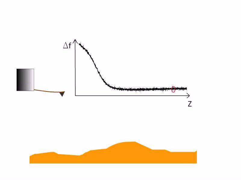 |
| Figure 2. The principle of atomic force microscopy in non-contact dynamic mode. Source: András Magyarkuti MSc defense (BME, Department of Physics, 2013). |
During low temperature AFM measurements the optical detection of the cantilevers movement is very challenging. Therefore it is practical to use a sensor which movement can be measured in an electrical way. The simple and cheap quartz tuning fork shown in Figure 1. is suitable to be used in an AFM device by attaching a sharp tip on one of its prongs because of the high quality factor of its resonance which ensures that a small force on the tip causes a measurable change in the resonance frequency. It is demonstrated in Figure 3. On the left side there is scanning tunneling microscope (STM) image of a gold coated nanostructure (the height of the tip was adjusted in a way that the tunneling current was constant), on the right side the same area was mapped with a tuning fork keeping the force (and the resonance frequency) constant between the sample and the tip. The main features of the two images are matching.
 |

|
| Figure 3. The topography of a gold coated surface measured in scanning tunneling and atomic force microscopy mode. Source: András Magyarkuti MSc thesis (BME, Department of Physics, 2013, in Hungarian). |
You can reach further information about scanning probe microscopy in Nanofizika tudásbázis, Nanoszerkezetek előállítási és vizsgálati technikái (Hungarian).
A simple model for the quartz resonator
The simplest model for an elastic piezoelectric system like the quartz resonator with one degree of freedom is an  mass which can move only in
  direction attached to a spring with an effective spring constant
  . The piezoelectric coupling can be described by the
![\[ \left(\begin{matrix} z \\ Q \end{matrix}\right) = \left(\begin{matrix} k^{-1} & s \\ s & C \end{matrix}\right)\cdot \left(\begin{matrix} F \\ U \end{matrix}\right)\]](/images/math/1/1/f/11f958437f7f14b356a0ec4a6acbb677.png)
matrix equation, where is the displacement,  is the charge on the electrodes of the resonator,
  is the force,
  is the voltage between the electrodes,
  is the displacement induced by a unit voltage when
  , is the effective spring constant when
  , and
, and  is the capacity of the system when . Since the conservation of the energy the determinant of the matrix in the equation is
  , which means
  . Due to this coupling the charge on the electrodes is proportional to the displacement of the system:
![\[Q = \alpha \cdot z\]](/images/math/d/6/8/d68a6dd0d6ac5afb20460b77f6918c90.png)
where  .
.
To describe the dynamics of the system one must consider the damping due to the drag of the fluid around it. If it is proportional to the velocity of the electrodes, then the mechanical equation of motion is
![\[m \ddot{z} = -kz - \gamma \dot{z} + \alpha U\]](/images/math/4/1/b/41bfd22c4cca1e76bbcaaa30639eb6ca.png)
where  is the damping ratio.
From  the current of the sensor is proportional to the velocity of the oscillator:
  . If we substitute this to the mechanical differential equation of motion, we get an equation what describes a series RLC circuit driven by voltage , and where the
  ,
,  and electrical parameters correspond to the , and mechanical parameters via the piezoelectric constant .
Finally, we should not forget about the capacitance of the electrodes of the system, which would be there even when the material between them is not piezoelectric. It appears in the model as a  capacity parallel to the RLC circuit as shown in Figure 4. This equivalent circuit describes the electric behaviour of quartz sensors in a very accurate way.
 |
| Figure 4. The electric equivalent circuit of quartz resonators. |
In this model the formula for the absolute value of complex impedance of a quartz resonator is
![\[|Z|=\frac{\sqrt{(A-\omega^2)^2+D^2 \omega^2}}{E \omega \sqrt{(B-\omega^2)^2+D^2\omega^2}}\]](/images/math/7/f/c/7fc534ab9c2d8cde6b2329a20361ad42.png)
![\[A = \frac{1}{L C}, \quad B = \frac{C + C_0}{C_0 C L}, \quad D = \frac{R}{L}\quad\text{and}\quad E = C_0.\]](/images/math/3/f/d/3fd1f03cc2084ba2c9ee208a8dd5c933.png)
Measurement tasks
1. Measure the impedance of the given parallel LC circuit in the function of frequency with a current bias. Determine the value of its resonance frequency, capacitance, inductance and the series resistance of the coil. Compare the measured curve with the theoretical calculation. For this:
- Write a computer program which connects to the lock-in via a GPIB port. The program should set the frequency of the output voltage in logarithmic steps between two given values, and register the
 and
and  or the and
  (or every 4) components of the signal on the input at every step.
- Take care about the correct setting of the time constant of the lock-in.
- Consider that the lock-in amplifiers output is a voltage bias, which means if the impedance on the output is considerably higher than
 then the output voltage is going to be independent from it. Design a current bias drive for the LC circuit, and choose its parameters in a way that the current of the LC-circuit doesn't change more than 1% during the frequency sweep.
2. Measure the resonance curve of the given capped quartz resonator with a voltage bias, and determine the value of its , , and parameters. For this:
- Instead of directly connect the resonator to the input of the lock-in use a series resonance.
- To get more precise frequency values use a Siglent function generator as a frequency source. Synchronize the the lock-in to the Siglent, and use the output of the lock-in as a voltage source (as before).
- Do the necessary modifications of the program written in task 1.
- Warning! The quartz oscillator can be damaged if it is driven with an excessive voltage at its resonance. Take care, that the amplitude of the drive if less than
 .
.
- Take care, that the oscillator returns to its steady-state very slowly if it was driven near to its resonance. Therefore after changing the frequency of the drive, it can take some time to get to the new steady-state of the system. Estimate the time constant of the decay of the vibration using the calculated quality factor of the system. Could you check easily if your measurement was slow enough by experiment? (So at every data point the earlier resonance of the oscillator is negligible compared to the new one.)
- Near to the resonance it is worthy to measure with a higher frequency resolution in linear steps. Due to the parallel capacitance their is an antiresonance next to the resonance, where the current of the oscillator is minimal. Observe this also.
- Which parameter of the oscillator can be easily determined from a wide range, logarithmic measurement?
3. With pliers carefully apply force to the sealing of the cap, open and remove it. Measure the resonance curve of this "uncapped" oscillator. Under the digital microscope apply some sort of glue (e. g. vacuum grease) on a prong of the tuning fork then attach small pieces of copper wire to it as it is shown on Figure 5. Measure the resonance curve of the oscillator at as much different values of the attached mass as it is possible. Determine how does the resonance frequency of the oscillator change in the function of the attached mass, then calculate the effective mechanical parameters (, and ) of the (empty) tuning fork.
- Explain what happened to the quality factor of the resonator after it was uncapped.
- When you put mass to the resonator its quality factor decreases, and under a too large load one cannot measure proper resonances. Use as little amount of the glue as possible to attach the copper wire pieces.
 |
| Figure 5. Setup to determine the tuning fork mechanical parameters. |
4. Az elektromos és mechanikai paraméterek (,, , , , ) ismeretében, a fent ismertetett egyszerű modell alapján számoljuk ki, hogy 1V egyenfeszültség hatására mekkora az oszcillátor elmozdulása. Ezen eredmény alapján adjunk becslést arra, hogy egy kvarc hangvillából készített atomerő-mikroszkóp szenzort a rezonanciafrekvencián milyen amplitudójú a.c. feszültséggel kell gerjeszteni ahhoz, hogy a mechanikai rezgési amplitudó két szomszédos atom tipikus távolságánál kisebb legyen!
Tools used in this lab
- SRS830 Lock-In + használati utasítás + tápkábel
- Siglent SDG1025 függvénygenerátor + használati utasítás (elektronikusan) + tápkábel
- GPIB <-> USB adapter + 1 GPIB kábel VAGY 1db soros port + kábel és 1db USB kábel a kommunikációhoz
- LC kör fém dobozban
- Kvarc oszcillátorok
- Ellenállásdekád
 -os lezáró
- 6db. közepes BNC-BNC kábel
- BNC T-elosztó
- Digitális mikroszkóp állvánnyal és csatlakozással a kvarc szenzorhoz
- Fogó a kvarc szenzor tokjának kibontásához
- Kvarc oszcillátorra felhelyezendő rézdrót
- Gillette-penge
- vákuumzsír a rézdrót felragasztásához
- Csipesz vagy hosszabb drót a kis drótdarabok és a vákuumzsír felhelyezéséhez
Supplementary information
- For testing the connection of the serial port one can use NI MAX (description in Hungarian). In the measurement controller program use the SerialPort object (example). In case of the SR830 lock-in amplifier set up the parameters with the following code:
serialPort1.PortName = "COM1";
serialPort1.DataBits = 8;
serialPort1.StopBits = StopBits.One;
serialPort1.Parity = Parity.None;
serialPort1.BaudRate = 9600;
serialPort1.NewLine = "\r";
serialPort1.DtrEnable = true;
serialPort1.Handshake = Handshake.None;
Note that, the baud rate can be changed on the amplifier, check it in its own menu. The serialPort1 is the name of an object, use it consequently. Do not forget to set up the PortName property in the proper way (the default value in case of the serial port of the motherboard is COM1).