Lock-in programming, investigation of a quartz sensor
Tartalomjegyzék |
Purpose of the measurement
The purpose of this measurement is to learn the usage and programming of the Stanford Research Systems SRS830 digital lock-in amplifier. For this purpose you're going to do a test measurement on an LC circuit, then you'll investigate and characterize a quartz sensor, similar to those that can be used in atomic force microscope (AFM) devices.
Nanophysical application of the quartz oscillators used in watches
An oscillator used in quartz watches is shown on the left side of Figure 1. Similar devices are being used to generate the clock signal in electronic circuits, their most important parameter is the resonance frequency. The tuning fork (TF) shaped oscillator in Figure 1. has a nominal resonance frequency of 32 768 Hz (= 215 Hz).
Due to the piezoelectric properties of crystalline quartz, the oscillation of the tuning fork can be excited using a voltage signal. A body shaped like this has several vibration modes, but the electrodes are prepared such a way to primarily excite the mode where the prongs vibrate mirror-symmetrically in the plane of the tuning fork. In this vibration mode, there is no force or angular momentum acting on the foot piece of the tuning fork, hence it is only weakly coupled to its environment. Therefore it can keep its resonance even in wristwatches where it is exposed to rapidly changing acceleration. Upon applying an AC signal to the electrodes, the crystal deforms periodically, generating a mechanical vibration. When the frequency of the applied voltage signal equals to the resonance frequency of the crystal, the amplitude of the vibration can become extremely high. In order to detect the mechanical vibration, the current between the electrodes can be measured, which is proportional to the velocity of the tuning fork's prongs. This current has a maximum value at the resonance frequency illustrated by the resonance curve on the right side of Figure 1.
 |
 |
| Figure 1. A quartz resonator used in watches (left) and its resonance curve (right). This curve is the amplitude of the current of the device in the function of the frequency of the constant amplitude excitation voltage. Source: András Magyarkuti MSc thesis (BME, Department of Physics, 2013, in Hungarian). | |
In a conventional atomic force microscope (AFM), a cantilever with a sharp tip placed at one end is approached to the surface of a sample. The movement of the cantilever is usually detected optically, by focusing a laser beam onto the cantilever and measuring the position of the reflected beam. When utilizing the so-called "dynamic mode", the cantilever is excited near to its resonance frequency, while maintaining a small distance between the tip and the sample. When the tip gets close enough to the sample, the force acting between the atoms at the apex of the tip and at the surface of the sample changes the resonance frequency of the cantilever. While sweeping the tip over the sample in the x and y directions the z height of the cantilever is continuously adjusted in a way that the resonance frequency of the vibration, and hence the force and the distance between the tip and the sample is kept constant, as it is shown in the video on Figure 2. (Note that the change in the resonance frequency is not proportional to the force itself, but to the derivative of the force with respect to the distance, which corresponds to the spring constant of the system.) By recording the z height as a function of the x and y positions, the topography of the sample can be investigated even with atomic resolution.
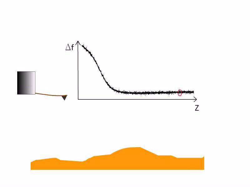 |
| Figure 2. The principle of atomic force microscopy in non-contact dynamic mode. Source: András Magyarkuti MSc defense (BME, Department of Physics, 2013). |
During low-temperature AFM measurements, the optical detection of the cantilever's movement can be challenging. Therefore it is practical to use such a sensor, whose movement can be detected electronically. The simple and cheap quartz tuning fork shown in Figure 1. is suitable to be used in an AFM device by attaching a sharp tip on one of its prongs. Due to the high quality factor of its resonance, a small force acting on the tip results in a measurable change in the resonance frequency. This is demonstrated in Figure 3. On the left side there is scanning tunneling microscope (STM) image of a gold-coated nanostructure (the height of the tip was adjusted in a way that the tunneling current was constant), on the right side the same area was mapped with a tuning fork keeping the force (and the resonance frequency) constant between the sample and the tip. The main features of the two images are matching.
 |

|
| Figure 3. The topography of a gold coated surface measured in scanning tunneling and atomic force microscopy mode. Source: András Magyarkuti MSc thesis (BME, Department of Physics, 2013, in Hungarian). |
You can find further information about scanning probe microscopy in Nanofizika tudásbázis, Nanoszerkezetek előállítási és vizsgálati technikái (Hungarian).
A simple model for the quartz resonator
The simplest model for an elastic piezoelectric system like the quartz resonator with one degree of freedom is a mass  which can move only in direction
  , attached to a spring with an effective spring constant
  . The piezoelectric coupling can be described by the
![\[ \left(\begin{matrix} z \\ Q \end{matrix}\right) = \left(\begin{matrix} k^{-1} & s \\ s & C \end{matrix}\right)\cdot \left(\begin{matrix} F \\ U \end{matrix}\right)\]](/images/math/1/1/f/11f958437f7f14b356a0ec4a6acbb677.png)
matrix equation, where denotes the displacement,  is the charge on the electrodes of the resonator,
  is the force,
  is the voltage between the electrodes,
  is the displacement induced by 1 V voltage when
  , is the effective spring constant when
  , and
, and  is the capacity of the system when . Since the conservation of the energy the determinant of the matrix in the equation is
  , which means
  . Due to this coupling, the charge on the electrodes is proportional to the displacement of the system:
![\[Q = \alpha \cdot z\]](/images/math/d/6/8/d68a6dd0d6ac5afb20460b77f6918c90.png)
where  .
.
To describe the dynamics of the system one must consider the damping due to the drag of the fluid around it. If it is proportional to the velocity of the electrodes, then the mechanical equation of motion is
![\[m \ddot{z} = -kz - \gamma \dot{z} + \alpha U\]](/images/math/4/1/b/41bfd22c4cca1e76bbcaaa30639eb6ca.png)
where  is the damping ratio.
From  the current of the sensor is proportional to the velocity of the oscillator:
  . If we substitute this to the mechanical differential equation of motion, we get an equation that describes a series RLC circuit driven by voltage , and where the
  ,
,  and electrical parameters correspond to the , and mechanical parameters via the piezoelectric constant .
Finally, we should not forget about the capacitance of the electrodes of the system, which would be there even when the material between them is not piezoelectric. It appears in the model as a  capacity parallel to the RLC circuit as shown in Figure 4. This equivalent circuit describes the electric behaviour of quartz sensors in a very accurate way.
 |
| Figure 4. The electric equivalent circuit of quartz resonators. |
In this model the formula for the absolute value of complex impedance of a quartz resonator is
![\[|Z|=\frac{\sqrt{(\omega_r^2 - \omega^2)^2 + \omega_r^2 \omega^2/Q^2}}{C_0 \omega \sqrt{(\omega_a^2 - \omega^2)^2 + \omega_r^2 \omega^2/Q^2}}\]](/images/math/c/a/3/ca318c3e7184586e890f4c191ce2a3ae.png)
![\[\omega_r = \frac{1}{\sqrt{L C}}, \quad Q = \frac{1}{R}\sqrt{\frac{L}{C}}, \quad\text{and}\quad \omega_a = \sqrt{\frac{C + C_0}{L C C_0}}.\]](/images/math/0/d/4/0d4b2a1392945ebfe2f1653a50767247.png)
Measurement tasks
1. Measure the impedance of the given parallel LC circuit as a function of frequency using a current bias. Determine the value of its resonance frequency, capacitance, inductance and the series resistance of the coil. Compare the measured curve with the theoretical calculation. For this:
- Write a computer program that communicates with the lock-in amplifier via a serial or GPIB port. The program should sweep the frequency of the output voltage signal between two given values, and record the (amplitude) and
 (phase shift) parameters of the measured signal at each step.
- Take care about the correct setting of the time constant of the lock-in.
- Consider that the lock-in amplifiers output is a voltage bias, which means if the load impedance is considerably higher than
 then the output voltage is going to be independent from it. Design a current bias drive for the LC circuit, and choose its parameters in a way that the current of the LC-circuit doesn't change more than 1% during the frequency sweep.
2. Measure the resonance curve of the given quartz oscillator (without opening the cap) using a voltage bias, and determine the value of its , , and parameters. For this:
- Use a series resistance for measuring the current, using the voltage input of the lock-in amplifier.
- To set the drive frequency more precisely, use a function generator as a frequency source. Synchronize the the lock-in to the function generator and use the output of the lock-in as a voltage source to drive the oscillator.
- Do the necessary modifications of the program written in task 1.
- Take care, that it takes time for the oscillator to return to its steady-state after it was driven near to its resonance. Therefore after changing the drive frequency, you have to wait some time to get to the new steady-state of the system. Estimate the time constant of the vibration decay using the calculated quality factor of the system. How could you easily check experimentally, whether your measurement was slow enough? (Whether at each measurement point, the previous excitation has already decayed and it is negligible compared to the vibration at the current frequency.)
- Measure the impedance of the oscillator with high frequency resolution, near its resonance. Due to the parallel capacitance there is an antiresonance next to the resonance, where the impedance of the oscillator is minimal. Don't forget to measure this part also.
3. Carefully apply force to the sealing of the cap, using pliers, to open and remove it. Measure the resonance curve of this "uncapped" oscillator. Estimate the mass of the ink left by a permanent marker on both prongs of a tuning fork.
- Explain what happened to the quality factor of the resonator after it was uncapped.
- To estimate the mass of the ink left by the marker, one should measure the resonance frequency of an empty tuning fork, then the same after its prongs are marked.
 |
Figure 5. Dimensions of the tuning fork:  . .
|
- The bending of a rectangular object (one prong of the oscillator) can be calculated as the following:
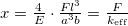 , where
  is the Young modulus, is the force and
  ,
,  ,
,  are the dimensions of the object. Besides that, at the resonance frequency:
 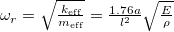 , for the quartz oscillator, where
 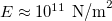 , and
, and  . Substitute
  to the second equation, and calculate the ratio of the effective mass and the actual mass of the prongs (using that
  is the mass).
- Calculate the masses at the resonance frequencies of the two cases (empty fork and marked fork) and calculate the mass of the ink.
Additional measurement tasks
4. Under the digital microscope, apply some sort of glue (e. g. vacuum grease) on one prong of the tuning fork then attach small pieces of copper wire to it as it is shown on Figure 5. Measure the resonance curve of the oscillator at as much different values of the attached mass as it is possible. Determine how does the resonance frequency of the oscillator change in the function of the attached mass, then calculate the effective mechanical parameters (, and ) of the (empty) tuning fork.
- When you put mass to the resonator its quality factor decreases, and under a too large load one cannot measure proper resonances. Use as little amount of the glue as possible to attach the copper wire pieces.
- To estimate the length of the wire pieces one can compare them to the width of a prong which is
 .
.
 |
| Figure 6. Setup to determine the tuning fork mechanical parameters. |
5. By the usage of the determined electrical and mechanical parameters, calculate how big is the displacement of the tuning fork ends when we apply  DC voltage on it (you can use the simple model above). By this result estimate the amplitude of AC voltage driving the quartz tuning fork on its resonance at which the amplitude of its mechanical vibrations is less than the typical distance of neighbouring atoms.
Tools used in this lab
- SRS830 Lock-In amplifier + user's manual + power cord
- Siglent SDG1025 function generator + user's manual + programming guide + power cord
- GPIB <-> USB adapter + GPIB cable OR serial port + USB cable
- LC circuit in a proper box
- quartz resonators
- resistance table
 BNC terminator
- 6 medium length BNC cable
- T branch for BNC cables
- digital USB microscope + stand + connection
- pliers for the opening of the cap of the tuning fork
- copper wire for the mechanical calibration
- razor blade or retractable knife blade
- some sort of glue (e. g. vacuum grease)
- tweezers to operate with the small pieces of wire
Supplementary information
For testing the connection of the serial port one can use NI MAX (description in Hungarian). In the measurement controller program use the SerialPort object (example). In case of the SR830 lock-in amplifier set up the parameters with the following code:
serialPort1.PortName = "COM1";
serialPort1.DataBits = 8;
serialPort1.StopBits = StopBits.One;
serialPort1.Parity = Parity.None;
serialPort1.BaudRate = 9600;
serialPort1.NewLine = "\r";
serialPort1.DtrEnable = true;
serialPort1.Handshake = Handshake.None;
Note that, the baud rate can be changed on the amplifier, check it in its own menu. The serialPort1 is the name of an object, use it consequently. Do not forget to set up the PortName property in the proper way (the default value in case of the serial port of the motherboard is COM1). Also, do not forget to open the port before the measurement, and close it afterwards.
Use the timer and tick events for programming the frequency sweep via the function generator and monitoring the amplitude and phase measured by the lock-in amplifier. Graph the amplitude and the phase as a function of the frequency, for that, use the 2-panel template project as a starting point.